Why diffusion draws seams on 40-megapixel photos, and how to give tiles a memory

A professional retouching file has 40 to 150 megapixels and a diffusion model works on one to four at a time, so every pipeline cuts the photo into tiles. That brings two problems: a visible step at tile borders, and a model that has no idea what it is looking at. This post covers why blending cannot remove the step, which memory mechanisms from video diffusion carry over from frames to tiles, why each tile should get the whole picture and its own coordinates, and what my first runs showed, failures included. I worked as a retoucher for over twenty years and am in my fourth year of making diffusion behave on files like these; the work belongs to the hi-res img2img research behind Happyin.ai. Revised in September 2026: corrections and later results carry that date.

Why everyone tiles

Retouching does not live at 2048 pixels a side. A Phase One IQ4 gives 14200×10600, a Hasselblad H6D-100c 11600×8700, a Canon R5 8192×5464, and all of it still needs skin, hair, colour, light and background work. Current models are native at 1024 to 2048: SDXL and SANA at 1024 (SANA was trained further, up to 4K), FLUX and Klein acceptably at 2048. Below 1024 quality drops and the tile count grows.

At tile 1024 with a small overlap, a 60 MP file is 75–80 tiles, 100 MP about 130, 150 MP about 190. Overlap is what hides seams, and it multiplies the count: the same 150 MP file is about 270 tiles at 25% overlap and about 540 at 50%. So 150+ tiles per image is a normal working case, and any mechanism whose cost grows with the square of the tile count is out before it starts. It will not fit in 80 GB of VRAM, and it will not fit in 192 GB either.

Why blending cannot remove seams

Overlap plus blending is the usual fix, and blending behaves differently at different frequencies. On smooth content (a sky gradient, skin tone, a soft falloff in a reflection on metal) a cross-fade hides a colour step well. On hair, stone, grain or fine scratches it fails one of two ways: a hard step stays at the border, or the texture is smeared, because inside the overlap you average two textures the model drew independently.

The smearing has a simple number behind it. Two uncorrelated textures of equal contrast, averaged 50/50, keep √0.5 of their contrast, about 71%. In the synthetic illustration below I measured 0.70 in the middle of the overlap.

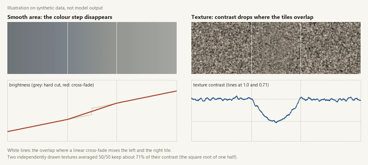
One knob cannot fix both: the harder you blend, the softer the colour seam and the flatter the texture along every tile border. And the colour step itself comes from tiles drifting independently. Nothing tells tile (3, 5) which colour tile (3, 4) chose.

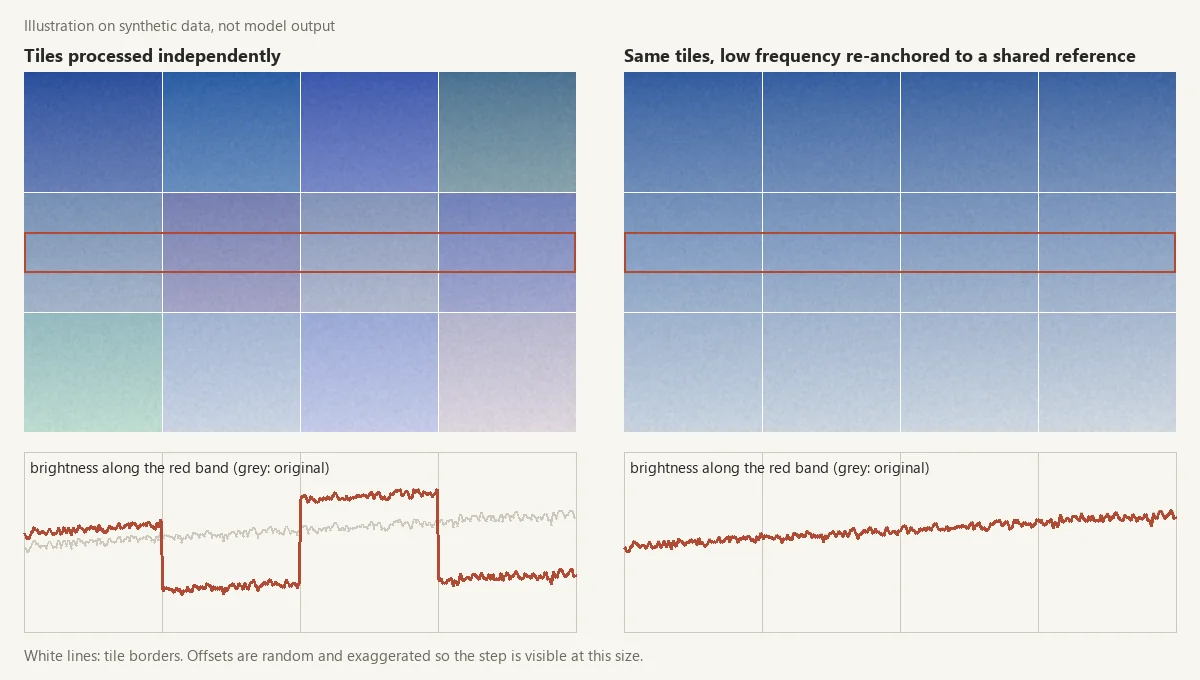
In this toy the largest step at a tile border falls from 18.5 levels of 255 to 0.5. The offsets are exaggerated, but the principle is the direction of this whole post: give every tile a reference it shares with its neighbours, and fix the low frequencies against that reference rather than against each other. ResMaster does a version of this for generation, aligning the low-frequency components of each patch with a low-resolution reference at every denoising step.

What a memory mechanism for tiles has to do

• Cost that does not grow quadratically with the number of tiles. Full 3D attention is out.
• Some use without retraining. Even partial inference-only use is a big advantage.
• Continuous, pixel-precise output. We retouch texture, we do not generate an aesthetic. Discrete-token models such as Cosmos, with its FSQ vocabulary of 64K, quantise fine detail away.
• A primitive I can lift out. Wan 2.1 (14B) and HunyuanVideo (13B) carry long video, motion control, audio sync and multi-shot composition; half of that solves problems a photo does not have, and I would pay for all of it in VRAM. SANA-Video, AnimateDiff, SVD and FramePack each isolate their memory primitive. And Apache 2.0 where possible, so the result can go into a product without negotiation.

The main axis I choose along is how a mechanism forgets finished tiles, so that 200 of them do not sit in VRAM with all their K/V tensors. A sliding window keeps the last few and is blind to anything far away. Geometric compression keeps neighbours at full resolution and distant tiles compressed, so the total converges. Accumulated state keeps no tiles at all, only two small running sums.

Idea one: video models remember frames, photo models do not

By "photo model" I mean an ordinary image-to-image diffusion model: SDXL, FLUX, Klein, SANA. When a video model generates frame 18, it also sees 17, 16, some early key frames, sometimes the first. That memory lives in the architecture (attention over the time axis, an accumulated state, a KV cache between chunks), and it is why backgrounds do not jitter and colour does not drift between frames.

A photo model processing tile (3, 5) gets its pixels and a text prompt. No neighbour to the left, none above, no idea this is one picture. Move the memory from the time axis to the spatial grid and you address the seams (tiles remember their neighbours' colour) and part of the semantics (the hair tile knows a neck starts below it, not fur). The video literature has eight architectural classes of memory, and not all of them survive the move to a plane:

type	mechanism	examples	for tiles
A · full 3D attention	every token sees every token	Wan	drop: quadratic, will not start at 64+ tiles
B · block linear attention	running sums S = Σ φ(K)ᵀV, Z = Σ φ(K)ᵀ	SANA-Video	primary: constant state
C · sliding window	attend to the last W frames	CausVid	backup: good locally, blind to distant tiles
D · factored space + time	temporal layers after each spatial layer	SVD, AnimateDiff	direct map: "across all frames" becomes "across all tiles"
E · anchor frame	every frame attends to an anchor	Rolling Forcing, StreamingT2V	add-on: an anchor tile aligns colour
F · geometric compression	near frames full, far ones compressed	FramePack	primary: neighbours full, diagonals 2×, distant 4×
G · cache sharing	features computed once, reused across steps	Ca2-VDM	add-on: compute neighbour features once
H · discrete tokens	FSQ vocabulary, next-token prediction	Cosmos	drop: incompatible with continuous pixel editing

Three of them matter.

B, block linear attention from SANA-Video. Each block (a frame there, a tile here) adds its keys and values to two accumulators, and the next block reads from the accumulators instead of from every previous token. The state does not grow with the number of blocks, so a hundred tiles cost what ten cost. SANA already uses linear attention in every layer, so the primitive is there for free.

Update, September 2026. The April version put this state at about 380 MB for SANA 1.6B, using a width of 2,304 and 28 layers. Both numbers were wrong for that model: 2,304 is the width of the text-encoder embeddings (caption_channels), and 28 layers belong to the 0.6B model. SANA 1.6B has 20 layers of 70 heads with 32 dimensions each (config), and its linear attention keeps S and Z per head, in fp32 (SanaLinearAttnProcessor2_0 in diffusers). That is 33×32 numbers per head, about 6 MB for all 20 layers. Even a crude count, one 2,240×2,240 matrix per layer in fp16, gives about 200 MB. The conclusion gets stronger: the state is constant in the number of tiles, and small.

D, factored space and time, as in SVD. SVD inserts temporal convolution and attention layers after every spatial layer of an SD 2.1 UNet: 656M new parameters out of 1,521M, so the video part is 43% of the model. (The Russian original said SDXL; the SVD paper says SD 2.1. Corrected in September 2026.) Mechanically it is a reshape: after a spatial block, (B·T, C, H, W) becomes (B·H·W, T, C), goes through temporal attention and comes back. Put the number of tiles in place of T, and "how does this pixel look in every frame" becomes "how does this position look in every tile". It is the most literal port, and I expected it to be the most fragile. AnimateDiff motion modules are the same idea, already trained and usable at inference, but capped at 32 frames, so 32 tiles.

F, geometric compression from FramePack (Lvmin Zhang, the author of ControlNet). Near frames enter the context at full density, far ones compressed harder, so the total converges to a fixed limit. For tiles: (3, 5) sees (2, 5), (3, 4), (3, 6) and (4, 5) at full density, diagonals at 2× compression, far tiles at 4×. The context stays the same whatever the photo size, so 16×16 grids work without the quadratic blow-up.

The nearest existing work goes in neighbouring directions. PatchVSR adapts a video model to patch-wise super-resolution, but its temporal attention stays inside a patch, across that patch's frames. Sliding Tile Attention speeds up attention in video DiTs 2.8–17× over FlashAttention-2; the sliding-tile idea came from there, but it is a speed result. (The April text called that range end-to-end; in the paper it is for attention. Corrected in September 2026.) FrescoDiffusion (March 2026) is the closest cousin: tiled denoising for 4K image-to-video, each tile fused against a low-resolution reference at every timestep. It generates video rather than editing a photo. I found no systematic experiment using video temporal attention as cross-tile attention for a still image across backbones.

A dataset of neighbours, not of tiles

Almost nobody writes about the dataset, and it is half of the task. To learn to remember neighbours, the model has to see sequences of neighbours. I use strips: one straight row or column through a photo, cut into tiles.

The source is a jewellery set I had to hand, about 52,500 photos. Jewellery concentrates everything naive tiling fails on: thin edges, refraction, reflective metal with uneven shadows, stones with fine texture. Each photo is cut at three scales (512, 768, 1024), with three overlaps (0%, 25%, 50%), in four directions. Only left-to-right and top-to-bottom strips are stored; the reversed ones come from np.flip in the loader. The reversal matters for block linear attention, because it is causal: a tile sees only the running summary of tiles before it, and trained left to right only, it has never seen any other walk.

On paper that is about 70 strips per photo and 3–4 million examples for the whole set. The pipeline is designed to stop at 400,000 stored strips, with tiles resized to 256×256 for the first round and the originals kept for a later re-cut. Checked in September 2026: according to its manifest, the one run so far cut 7,368 strips from 100 photos, 74 per photo, close to the estimate.

Building it gave the most useful observation of the week: strips cross object boundaries. On one 5184×3456 photo, row 4 at scale 512 goes skin, skin, skin, fingertip, bracelet beads. At 24 to 60 frames a second, consecutive video frames are 17 to 42 ms apart, with small motion and smooth optical flow; neighbouring tiles jump from skin to metal in one step. A stride of half a tile makes a strip behave like a slow pan, and the final set mixes all three overlaps, from hard jumps to smooth pans.

What I ran in April

At the time of the original post, only SANA. It was trained at 512, then 1024, 2K and 4K, so a 1024 tile is native, and linear attention is already in the backbone. I ran a small training on test strips at tile 1024 with two questions: does the loss converge, and does the mechanism transfer from the time axis to the spatial plane at all. The loss converged, and the model learned to reconcile neighbouring tiles the way it used to reconcile neighbouring frames. I did not publish numbers from a test run and I still do not.

Update, September 2026. Re-reading the project repository, I found no log of that SANA training in it; the loss curves it keeps belong to two other ports. So treat the SANA sentence above as my April report, not as evidence. What the run notes of that week do hold: at inference, switching SANA's accumulated state on changed the output by a mean of 19.5 levels of 255, where the sanity check halts below 0.5. The mechanism is not a silent no-op, which is much less than "better". The two other ports were fine-tuned on tile sequences from a separate set of about 7,000 photos of 1024 px and larger. SDXL with SVD-style attention across tiles: the 100-step moving average of the loss fell by about 40%, and predictions had recognisable structure but a diagonal moiré aligned to the tile grid, which I attribute to the way my implementation mean-pools keys and values across tiles. AnimateDiff motion modules on SD 1.5: the weights changed (Frobenius norm of the update 15.28), yet outputs before and after fine-tuning looked almost identical. The notes disagree with each other on how far that loss fell, so I leave the number out. I read the identical outputs as a negative result for motion modules on tiles, and my working explanation is the content jumps above: the modules carry a smooth-motion prior that photos do not satisfy. Both were under-trained snapshots, so the numbers are a lower bound, not a result.

Idea two: give each tile the whole picture and its position

If you cut a 6000×4000 photo into tiles, you are holding the whole image, and not using it is strange. Downscale it in latent space and feed it with every tile as extra channels into the first convolution. Add the tile's position as two more channels, (x, y) ∈ [−1, 1], so tile (3, 5) knows it is (3, 5) and not some 512 pixels in the void. PatchVSR does both for video super-resolution: a global branch sees the resized full video, and the patch location is injected into the model.

What position is worth: PaDIS

PaDIS (Hu et al., NeurIPS 2024) trains a diffusion prior on patches only and concatenates two positional arrays to every patch: the x and y coordinates of each pixel in the full image, scaled to [−1, 1], with no noise added to them. The ablation in their appendix (Table 6, CT reconstruction) is blunt: 33.57 dB PSNR with position, 23.25 dB without, 24.51 dB without position even when initialised from a baseline reconstruction. The authors write that the network "completely failed to learn the patch-based prior". Ten decibels is the gap between working and not working.

Two caveats before borrowing that number. It is CT, not photographs, and a pixel-space model trained from scratch on patches. Nobody has measured what coordinates add to a pretrained latent model on 40 MP retouching; that experiment is first on my list and not done.

Why it matters is easy to see. Without position, one function has to restore every patch with no way to tie knowledge to a place ("faces usually here, sky gradient there"), so it averages, and the average looks like noise. Two numbers per pixel cost almost nothing, and almost no tiled pipeline feeds them, probably because a pretrained model has a fixed input width and every extra channel means training.

Three levels of what a tile should know

level	meaning	who does it
geometric	"I am tile (3, 5) of an 8×8 grid"	PaDIS coordinate channels
visual	"the whole picture looks like this"	DemoFusion, FreeScale, DC-VSR, ResMaster
semantic	"this is skin, next to it is hair, do not invent an ear"	AccDiffusion v2, a VLM caption per tile

Tiled VAE out of the box gives level zero: pixels and one global prompt.

For the visual level, two things work: a downscaled VAE latent of the whole image into the first convolution (keeps spatial structure, colour, lighting), or a 64-dimensional vector of global statistics (mean colour, exposure, white balance) modulating AdaLN-Zero in every block, which is cheaper but carries no spatial information. A CLIP image embedding through IP-Adapter does not work well: a vector without spatial axes cannot say "this tile's top edge is dark blue sky, its bottom edge pale".

I measured that rather than assumed it. A counterfactual probe on SDXL, real preview against a random-noise preview at adapter scale 0.4, gave a mean difference of 0.0066 per pixel (maximum 0.26), under the 0.02 threshold below which I call a signal decorative. The image encoder fires on every call, so the adapter runs and changes almost nothing. My guess in April was an encoder mismatch: the adapter was trained on bigG ViT image embeddings, while the setup used the standard SDXL pair of CLIP-L and CLIP-G.

Update, September 2026. That guess is still untested. The probe record shows a second candidate: the whole picture reaches the adapter as 224×224 pixels, which on its own limits what it can carry.

For the semantic level, the direct route is a caption per tile from a VLM such as Florence-2, about 50 ms a tile: a tile with a shoulder and hair gets "skin and hair, no fur", and a hallucinated fur texture contradicts its own prompt. The cheaper variant I want to try is one description for the whole picture, with the weight of absent tokens lowered in each tile, so the sky tile mutes face, hair and metal. AccDiffusion v2 builds patch-level prompts from one image prompt in a similar spirit. Untested on my side.

Put together, a tile's input is its own latent, two coordinate channels, the downscaled latent of the whole picture and an optional segmentation mask. The new input weights must start at zero. Otherwise at step zero the model sees its normal input plus random weights, and the pretrained behaviour breaks on the first forward pass. With zero-init it starts identical to the backbone and learns to use the new channels gradually, the same trick as the zero convolutions in ControlNet.

# Illustration, not production code: widen a pretrained first convolution
# so each tile can also receive its coordinates and a global preview.
import torch
import torch.nn as nn

def widen_first_conv(conv: nn.Conv2d, extra: int) -> nn.Conv2d:
    new = nn.Conv2d(conv.in_channels + extra, conv.out_channels,
                    conv.kernel_size, conv.stride, conv.padding)
    with torch.no_grad():
        new.weight.zero_()                     # new channels start silent
        new.weight[:, :conv.in_channels] = conv.weight
        new.bias.copy_(conv.bias)
    return new

def coord_channels(box, full_w, full_h, h, w):
    x0, y0, x1, y1 = box                       # tile position in the full image, px
    xs = torch.linspace(x0, x1, w) / full_w * 2 - 1
    ys = torch.linspace(y0, y1, h) / full_h * 2 - 1
    gy, gx = torch.meshgrid(ys, xs, indexing="ij")
    return torch.stack([gx, gy])               # (2, h, w), values in [-1, 1]

Bugs that looked like results

Added in September 2026 from the project log of that week. Two bugs and one near miss taught me more than the runs did.

• Coordinates that did nothing. The function meant to add coordinate channels returned the image unchanged and was never called, while its docstring promised concatenation into the first convolution. An explicit ablation showed a difference of exactly 0.0. The fix for the training-free path, a position-dependent colour tint, was then too weak: ±1% is about 2.5 levels of 255, below JPEG noise. It went up to 5%, about 13 levels.
• A near miss: an adapter switched off by the attention backend. Code review of the combined pipeline found xformers enabled after load_ip_adapter(). If xformers falls back, that replaces IP-Adapter's attention processors with plain ones, with no error, and the adapter simply stops having any effect. The reviewer rated it likely (85%); nothing showed it had happened in a run. The order is now VAE tiling, xformers, then the adapter, with a check of the processor class afterwards.
• A probe that passed by accident. The first AnimateDiff probe read the leading dimension of 4-D tensors as the frame axis. Classifier-free guidance doubles that dimension, the count came out as twice the number of tiles, and the probe said OK. It now reads only 5-D tensors, where the frame axis is real.

The lesson is now a project rule: no silent fallbacks, and every probe gets a control mode that deliberately breaks the mechanism and must come back FAIL. A probe never seen failing proves nothing. Retrofitting a control mode to each of the eleven verification techniques in the project is still open. How I write rules like these for agents is in the post about my CLAUDE.md.

Bonus idea: fewer tiles instead of smarter ones

A hypothesis with no runs behind it. Detail Daemon (and its ComfyUI port) reshapes the sigma schedule so the late, low-noise steps add more detail, without retraining.

The first half of the denoising steps handles low frequencies: colour distribution, composition, large shapes. That could run on a downscaled version in one pass, with no tiles and no low-frequency seams. The second half adds detail, and Detail Daemon does it through the schedule rather than a recursive re-denoise. If this holds, half the steps are cheap and seam-free, and tiling survives only in the detail phase, probably still needed above about 2048 a side, since attention maps at 4096×4096 do not fit in 80 GB either. The step-saving experiment (five methods at five step budgets, detail measured by Laplacian variance, high-frequency energy and spectral slope) is written and not run. The tiling and frequency nodes I do use in production graphs are in the post on custom ComfyUI nodes and on /comfyui/.

What none of this proves

• The full ablation is not done. The SANA run I reported in April is neither a full training nor a comparison against baselines, and its log is not in the repository. Seam PSNR, the ΔE ratio between tile borders and interiors, and HF-SSIM on skin and hair masks are unmeasured.
• I do not know which architecture wins. Block linear attention on SANA should win on memory, a cached Klein on quality, SVD-style attention is the most direct port. Which wins on a real ablation, I will not guess.
• I do not know how it scales. Every probe ran on 3×3 to 7×7 grids; a 100-tile grid needs FramePack-style compression or a sliding window.
• The semantic level is untested, and the Detail Daemon idea is a sketch.

Update, September 2026. None of this has changed. The last experiment commits in the project are from 26 April. In May I fixed a latent crash in a probe before it could cost GPU time, and set the project up for long runs: a feature list, a problem log, and a syntax gate that must pass before any GPU is rented. Checking for this update, I found that work still uncommitted on disk, which breaks my own rule that git is the source of truth. The next step is the same as in April: one GPU session that re-runs every fixed hypothesis with its probe, then the ablation. The second part of this series has not been published, and the code repository is still private. Read everything above as hypotheses with a few early signals.

What I would do differently

• Negative controls from the first day. Both bugs above are the kind a control run catches at once.
• Look at the strips before training on them. The content jumps were noticed after the first two fine-tunes had already run.
• One change per comparison. The first run of the global-preview method against the baseline differed in sampler, strength, seed, image size and negative prompt at once, so it said nothing about the preview. The fix was to align all of them and add a run with the preview switched off.